It’s a probabilistic technique (metaheuristic) used in local search algorithms for approximating the global optimum of a given function, especially when there is a lot of local optimum. Like every local search techniques, it starts with a possible solution of the problem, but it tries to move to a better point in the solution space probabilistically.

Background
The original idea of the simulated annealing was proposed in the 50’s while its application in real optimization problems occurred in the 80’s. It is a highly suitable search methodology for any non-convex optimization problem. From the physical point of view annealing is the process by which a solid, brought to a fluid state by heating at high temperatures, is brought back to solid or crystalline state, at low temperatures, gradually controlling and reducing the temperature. At high temperatures, the atoms in the system are in a highly disordered state and therefore the energy of the system is high. To bring back such atoms into a highly (statistically) ordered crystalline configuration, the temperature of the system must be lowered. Rapid reductions in temperature can cause defects in the crystal lattice with consequent metastability. Annealing avoids this phenomenon by proceeding with a gradual cooling of the system, bringing it to an overall excellent stable structure.
Main idea of the algorithm
Given a feasible solution of the problem, a successor is randomly chosen in its neighborhood, whose value could be less or more greater than the current. The probability of moving into a neighbor worse than the current decreases over time. Without loss of generality let’s assume we are in a maximization problem and that $V_c$ is the value of the current solution $c$ and $V_s$ of its successor $s$. The two scenarios are:
$V_s > V_c$ we find a better point, so $s$ become our new current solution;
$V_s \leq V_c$ we find a point that is currently worst, but that could in future lead us to the global optimum. Indeed, a worse point is not discarded a priori because it could make us leave a local optimum. So we accept $s$ in a probabilistic way:
Let $X_{cs}$ be a binary random variable with values: $1$ if we update solution $c$ with $s$ and $0$ otherwise. The probabilistic distribution is $P(X_{cs} = 1) = e^{\frac{\Delta V}{T}}$. Where $\Delta V = V_s - V_c$ and $T$ is the cooling temperature.
The idea of $\Delta V$ and $T$ is:
- $\Delta V$ is always negative because we subtract $V_c$ from $V_s$ and $V_s \leq V_c$. More negative $\Delta V$ is, less is the probability we’ll chose $s$ as a successor of $c$. On the other hand more similar $s$ is to $c$ more probable is that we’ll update the current point;
- $T$ starts with a positive value and it decreases over time. In the exponential function high values of $T$ lead us to accept worse values of the current more frequently. Indeed, it makes sense “try” worse solutions at the beginning of the iterations than at the end when we would like to obtain the global optimum. Temperature merely serves as a hyperparameter that implicitly defines the region of space explored by the algorithm. At high temperatures, the algorithm can cross almost all the space of admissible solutions since bad solutions are easily accepted. Then, by lowering the temperature, the algorithm is confined to increasingly restricted regions.
Pseudocode
There are a lot of possible different implementations of Simulated Annealing and these differ on:
- the way in which each parameters and hyperparameters are initially instantiated. The choice of the best values, for the problem under consideration, may take a lot of time;
- the function used to find a neighbour solution of the current one;
- the choice of an appropriate temperature reduction scheme which determines when and how much reduce it;
- the initial feasible solution from which the algorithm starts;
- the stop criteria of the main loop.
Here a possible implementation:
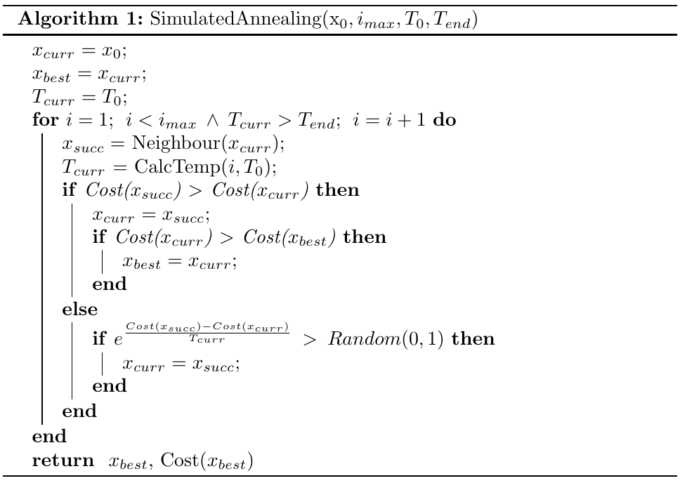
In this pseudocode at each iteration of the for loop we update the current temperature $T_{curr}$. Others implementations use an inner loop and generate multiple successors for each temperature value in order to approximate well the Boltzamann distribution. This improvement leads to a better solution, but increases the computational time. Another important thing about the temperature is how to update it. Reducing the temperature too quickly causes the possibility that the algorithm remains confined in a local optimum. On the other hand, reducing the temperature very slowly will result in an increase in the calculation time. There are essentially two temperature cooling schemes: the geometric one and the logarithmic one.
A different stop criteria than the one used in this pseudocode is to check whether the value of the best solution is close to theoretical global value, or to check when the last update of $x_{curr}$ occured.
One last thing about the pseudocode is that the we can use every neighbour search we want, on the condition that it’s fast and it obtains only feasible solutions of the problem.
Conclusion
At high temperatures, the algorithm behaves more or less like a random search. The research jumps from one point to another of the solution space by identifying the areas in which it is most likely to identify the overall optimum. At low temperatures, Simulated Annealing is similar to steepest descent methods.
This algorithm converges to the global optimum with a probability arbitrary close to $1$, but in a time that could be exponential. Conversely, using the Simulated Annealing as heuristic technique, its asymptotic behavior can be approximated in a polynomial time.
Author: Lorenzo Sciandra